Recommendation Systems
Introduction
Recommendation systems have become an integral part of our daily digital experiences. Whether shopping online, streaming movies, listening to music, or browsing social media, these algorithms work behind the scenes to provide personalized content. They analyze user interactions and preferences to suggest products, movies, articles, and more, enhancing user experience and engagement. Companies like Amazon and Netflix rely heavily on these algorithms to drive sales and viewer retention, showcasing the immense financial benefits of recommendation systems.
Here are some key statistics highlighting the importance of recommendation systems:
- Amazon: Approximately 35% of what consumers purchase on Amazon comes from product recommendations. This showcases the system's effectiveness in driving sales by suggesting relevant products to customers.
- Netflix: Over 75% of what users watch on Netflix is driven by recommendations. Netflix's recommendation engine plays a crucial role in keeping viewers engaged and subscribed.
- E-commerce Revenue: Recommendation systems are responsible for significant portions of revenue in e-commerce. For example, BestBuy experienced a 23.7% growth attributed to implementing a recommendation system.
- User Engagement: Companies that implement recommendation systems often see higher user engagement and satisfaction. Users are more likely to stay on the platform longer and interact with more content when it is personalized to their tastes.
Collaborative Filtering and Content-Based Filtering
Collaborative Filtering
Collaborative filtering is a popular technique that makes recommendations based on the preferences of similar users. If user A has the same opinion as user B on an item, A is more likely to share B's opinion on a different item than a randomly chosen user.
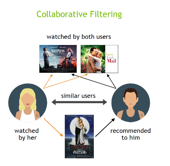
There are two main types of collaborative filtering:
- User-Based Filtering: Recommends items to a user based on items liked by similar users.
- Item-Based Filtering: Recommends items similar to those the user has liked in the past.
Similarity Calculation:
Pearson Correlation: Measures the linear relationship between two sets of data, accounting for mean and variance. It's defined as:
\[ \text{Pearson}(x, y) = \frac{\sum_{i \in I_{xy}} (r_{x,i} - \bar{r}_x) (r_{y,i} - \bar{r}_y)}{\sqrt{\sum_{i \in I_{xy}} (r_{x,i} - \bar{r}_x)^2} \sqrt{\sum_{i \in I_{xy}} (r_{y,i} - \bar{r}_y)^2}} \]
where \(I_{xy}\) is the set of items rated by both users \(x\) and \(y\).
Cosine Similarity: Measures the cosine of the angle between two vectors in a multi-dimensional space:
\[ \text{Cosine}(x, y) = \frac{\sum_{i} r_{x,i} \cdot r_{y,i}}{\sqrt{\sum_{i} (r_{x,i})^2} \sqrt{\sum_{i} (r_{y,i})^2}} \]
Matrix Factorization
Matrix factorization is a powerful technique used in collaborative filtering to discover latent factors influencing user-item interactions.
Singular Value Decomposition (SVD):
SVD decomposes a user-item interaction matrix \(R\) into three matrices:
\[ R = U \Sigma V^T \]
- \(U\) is an \(m \times k\) matrix where each row represents a user in the latent factor space.
- \(\Sigma\) is a \(k \times k\) diagonal matrix with singular values representing the strength of each latent factor.
- \(V\) is an \(n \times k\) matrix where each row represents an item in the latent factor space.
Content-Based Filtering
Content-based filtering is a recommendation system technique that recommends items to users based on the similarity between the items. This method leverages the attributes of items to make recommendations. For instance, in a music recommendation system, the attributes could include genre, artist, tempo, etc.
K-Nearest Neighbors (KNN) in Content-Based Filtering
K-Nearest Neighbors (KNN) is a popular algorithm used in content-based filtering. It works by finding the most similar items to a given user based on their attributes.
In this scenario, the similarity metric is Euclidean distance. This works by finding the magnitude of a straight line between two points in an N-dimensional space.
The Euclidean distance between two items with feature vectors \(x\) and \(y\) is given by:
\[ d(x, y) = \sqrt{\sum_{i=1}^n (x_i - y_i)^2} \]
where \(n\) is the number of features.
From there, identify the \(K\) nearest neighbors by finding the items with the smallest Euclidean distances and then recommend the \(K\) items to the user.
Introduction to Neural Collaborative Filtering (NCF)
Traditional matrix factorization uses an inner product to model user-item interactions, which may not capture complex patterns. Neural Collaborative Filtering (NCF) addresses this by using a neural network to learn the interaction function, allowing for non-linear transformations.
Architecture:
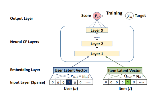
- Input Layer: Encodes user and item IDs as one-hot vectors.
- Embedding Layer: Maps one-hot vectors to dense latent representations.
- Neural CF Layers: Multiple hidden layers to model non-linear interactions.
- Output Layer: Produces the predicted interaction score \(\hat{y}_{ui}\).
Mathematical Formulation of NCF
Input Representation:
One-hot encoding of users \(u\) and items \(i\). Embedding vectors \(p_u\) and \(q_i\) are obtained from embedding matrices \(E_u\) and \(E_i\):
\[ p_u = E_u \cdot x_u, \quad q_i = E_i \cdot x_i \]
Interaction Function:
Modeled by a neural network with multiple layers:
\[ \hat{y}_{ui} = \phi_{\text{out}} \left( \phi_L \left( \ldots \phi_2 \left( \phi_1 \left( p_u, q_i \right) \right) \ldots \right) \right) \]
Each layer \(\phi\) typically applies a fully connected layer with a non-linear activation function, such as ReLU.
Detailed Computations in NCF
Embedding Layer: Transforms sparse input vectors into dense embeddings:
\[ p_u = E_u \cdot x_u, \quad q_i = E_i \cdot x_i \]
Hidden Layers: Compute activations using non-linear functions:
\[ h_1 = \sigma \left( W_1 \cdot \left[ p_u; q_i \right] + b_1 \right) \]
For subsequent layers:
\[ h_{l+1} = \sigma \left( W_{l+1} \cdot h_l + b_{l+1} \right) \]
Output Layer: Final prediction:
\[ \hat{y}_{ui} = \sigma \left( W_{\text{out}} \cdot h_L + b_{\text{out}} \right) \]
Training NCF
Objective Function: Use log loss for implicit feedback:
\[ L = - \sum_{(u,i) \in Y \cup Y^-} \left( y_{ui} \log \left( \hat{y}_{ui} \right) + \left( 1 - y_{ui} \right) \log \left( 1 - \hat{y}_{ui} \right) \right) \]
Where \(Y\) is the set of observed interactions, and \(Y^-\) is the set of negative samples.
Optimization: Optimize using Stochastic Gradient Descent (SGD) or Adam, with backpropagation to update model parameters.
Conclusion
In summary, this article explored the development and intricacies of recommendation systems, from traditional collaborative filtering and matrix factorization to the advanced Neural Collaborative Filtering (NCF). Collaborative filtering methods rely on user behavior similarities, while matrix factorization uncovers latent factors to improve recommendation accuracy. NCF leverages deep learning to model complex, non-linear interactions, offering significant improvements over traditional methods.